← All notebooks

December 1, 2021 4 min read

Principal Component Analysis

Step-by-step implementation of Principal Component Analysis (PCA) Method.

PCADimension ReductionSklearnPython

PCA¶

In [1]:

import matplotlib.pyplot as pltfrom mpl_toolkits.mplot3d import Axes3Dfrom sklearn import datasetsfrom sklearn.decomposition import PCAfrom numpy import linalg as LAimport numpy as np

In [2]:

# Datasetiris = datasets.load_iris()X_raw = iris.data.T    y = iris.target

In [3]:

X = X_raw - X_raw.mean(axis=1).reshape(4,1)   #data is centeredC = (1/X.shape[1]) * X @ X.T     #covariance matrixlmbd, U = LA.eigh(C)k = 2                     #Number of dimension to be reducedmask = np.argsort(lmbd)   #lambdas are sorted and highest k lambdas are used, others are eliminatedmask = np.flip(mask)      #to make the mask descending ordersorted_U = U[:, mask]         #Columns of U are reordered using masksorted_lmbd = lmbd[mask]      #lambdas are reorderedreduced_U = sorted_U[:,:k] H = reduced_U.T @ X

In [4]:

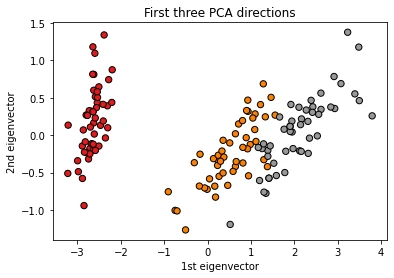
ax = plt.gca()H[0,:] = H[0,:] * -1ax.scatter(H.T[:, 0], H.T[:, 1],  c=y,           cmap=plt.cm.Set1, edgecolor='k', s=40)ax.set_title("First three PCA directions")ax.set_xlabel("1st eigenvector")ax.set_ylabel("2nd eigenvector")plt.show()

Using Sklearn library¶

In [5]:

ax = plt.gca()X_reduced = PCA(n_components=2).fit_transform(iris.data)ax.scatter(X_reduced[:, 0], X_reduced[:, 1],  c=y,           cmap=plt.cm.Set1, edgecolor='k', s=40)ax.set_title("First three PCA directions (using sklearn PCA function)")ax.set_xlabel("1st eigenvector")ax.set_ylabel("2nd eigenvector")plt.show()

PCA with Detailed Explanations¶

In [6]:

X_raw = iris.data.T    # Zy_raw = iris.target

Data centering: $$\vec \mu = \frac{1}{N} \sum_i \vec z_i$$ where N is the number of data
$$\vec x_i = \vec z_i - \vec \mu $$

In [7]:

X = X_raw - X_raw.mean(axis=1).reshape(4,1)   #data is centeredX.shape

Out[7]:

(4, 150)

In [8]:

# Manual implementationC = (1/150) * X @ X.Tprint("C:\n", C)# Check using numpycov =  np.cov(X, bias=True)print("\nnp.cov:\n", cov)

C:
 [[ 0.68112222 -0.04215111  1.26582     0.51282889]
 [-0.04215111  0.18871289 -0.32745867 -0.12082844]
 [ 1.26582    -0.32745867  3.09550267  1.286972  ]
 [ 0.51282889 -0.12082844  1.286972    0.57713289]]

np.cov:
 [[ 0.68112222 -0.04215111  1.26582     0.51282889]
 [-0.04215111  0.18871289 -0.32745867 -0.12082844]
 [ 1.26582    -0.32745867  3.09550267  1.286972  ]
 [ 0.51282889 -0.12082844  1.286972    0.57713289]]

In [9]:

# LA.eigh(C) function can be used when the data is symmetric real data.Otherwise, use LA.eig(C). Note: eigh is faster than eig functionlmbd, U = LA.eigh(C)print("lmbd: ", lmbd)print("\nU matrix:\n", U)

lmbd:  [0.02367619 0.0776881  0.24105294 4.20005343]

U matrix:
 [[ 0.31548719  0.58202985  0.65658877 -0.36138659]
 [-0.3197231  -0.59791083  0.73016143  0.08452251]
 [-0.47983899 -0.07623608 -0.17337266 -0.85667061]
 [ 0.75365743 -0.54583143 -0.07548102 -0.3582892 ]]

Checking an equality: $$C \vec u_j = \lambda_j \vec u_j$$

In [10]:

#For j=0left_eq = C @ U[:,0] print("C * u_j:\n", left_eq)right_eq = lmbd[0] * U[:,0]print("\nlambda_j * u_j:\n", right_eq)

C * u_j:
 [ 0.00746954 -0.00756983 -0.01136076  0.01784374]

lambda_j * u_j:
 [ 0.00746954 -0.00756983 -0.01136076  0.01784374]

$U^T U = I \iff U^T=I^{-1}$

In [11]:

#Check the left equationprint(np.round(U.T @ U, 3))

[[ 1. -0.  0. -0.]
 [-0.  1.  0. -0.]
 [ 0.  0.  1. -0.]
 [-0. -0. -0.  1.]]

$$C = U \Lambda U^T$$

In [12]:

print("C:\n", C)print("\n U @ Lambda @ U.T:\n", U @ (lmbd * np.eye(lmbd.shape[0])) @ U.T)

C:
 [[ 0.68112222 -0.04215111  1.26582     0.51282889]
 [-0.04215111  0.18871289 -0.32745867 -0.12082844]
 [ 1.26582    -0.32745867  3.09550267  1.286972  ]
 [ 0.51282889 -0.12082844  1.286972    0.57713289]]

 U @ Lambda @ U.T:
 [[ 0.68112222 -0.04215111  1.26582     0.51282889]
 [-0.04215111  0.18871289 -0.32745867 -0.12082844]
 [ 1.26582    -0.32745867  3.09550267  1.286972  ]
 [ 0.51282889 -0.12082844  1.286972    0.57713289]]

In [13]:

k = 2   #Number of dimension to be reducedmask = np.argsort(lmbd)   #lambdas are sorted and highest k lambdas are used, others are eliminatedmask = np.flip(mask)   #to make the mask descending ordersorted_U = U[:, mask]         #Columns of U are reordered using masksorted_lmbd = lmbd[mask]      #lambdas are reorderedreduced_U = sorted_U[:,:k] print("mask = ", mask, "\n")print("U:\n", U, "\n")print("sorted_U:\n", sorted_U, "\n")print("sorted_lmbd:\n",sorted_lmbd, "\n")print("reduced_U:\n", reduced_U, "\n")H = reduced_U.T @ Xprint("H.shape: ", H.shape)print("H[:,0]: ", H[:,0])

mask =  [3 2 1 0] 

U:
 [[ 0.31548719  0.58202985  0.65658877 -0.36138659]
 [-0.3197231  -0.59791083  0.73016143  0.08452251]
 [-0.47983899 -0.07623608 -0.17337266 -0.85667061]
 [ 0.75365743 -0.54583143 -0.07548102 -0.3582892 ]] 

sorted_U:
 [[-0.36138659  0.65658877  0.58202985  0.31548719]
 [ 0.08452251  0.73016143 -0.59791083 -0.3197231 ]
 [-0.85667061 -0.17337266 -0.07623608 -0.47983899]
 [-0.3582892  -0.07548102 -0.54583143  0.75365743]] 

sorted_lmbd:
 [4.20005343 0.24105294 0.0776881  0.02367619] 

reduced_U:
 [[-0.36138659  0.65658877]
 [ 0.08452251  0.73016143]
 [-0.85667061 -0.17337266]
 [-0.3582892  -0.07548102]] 

H.shape:  (2, 150)
H[:,0]:  [2.68412563 0.31939725]

In [14]:

# To getter a better understanding of interaction of the dimensions# plot the first three PCA dimensionsax = plt.gca()H[0,:] = H[0,:] * -1    # Since sklearn multiplies the first dimension with -1, I multiplied with -1 to compare with my resultax.scatter(H.T[:, 0], H.T[:, 1],  c=y_raw,           cmap=plt.cm.Set1, edgecolor='k', s=40)ax.set_title("First three PCA directions")ax.set_xlabel("1st eigenvector")ax.set_ylabel("2nd eigenvector")plt.show()

In [15]:

ax = plt.gca()X_reduced = PCA(n_components=2).fit_transform(iris.data)ax.scatter(X_reduced[:, 0], X_reduced[:, 1],  c=y_raw,           cmap=plt.cm.Set1, edgecolor='k', s=40)ax.set_title("First three PCA directions (using sklearn PCA function)")ax.set_xlabel("1st eigenvector")ax.set_ylabel("2nd eigenvector")plt.show()

Average Truncation Error¶

$$\vec x_i \approx \sum_{j=1}^k \vec u_j h_{ji} = \vec y_i \iff X \approx U_k H_k$$ where y is transformation of reduced X to original space

There are 2 different calculation of truncation error:

1. Norm square of difference between y and original centered data $$\epsilon = \frac{1}{N} \sum_i ||\vec x_i - \vec y_i ||^2$$
2. (sum of eliminated lambdas) $$\epsilon = \sum_{j=k+1}^m \lambda_j$$

In [16]:

H = reduced_U.T @ Xy = reduced_U @ H# There are 2 different calculation of truncation errortrunc_err_1 = ((X - y)**2).sum() / X_raw.shape[1]print("trunc_err_1 = ", trunc_err_1)trunc_err_2 = sorted_lmbd[k:].sum()print("trunc_err_2 = ", trunc_err_2)

trunc_err_1 =  0.10136429572959302
trunc_err_2 =  0.10136429572959307

In [17]:

print(sorted_lmbd)print(sorted_lmbd[k:])sorted_lmbd[k:].sum()

[4.20005343 0.24105294 0.0776881  0.02367619]
[0.0776881  0.02367619]

Out[17]:

0.10136429572959307