← All notebooks

July 20, 2022 5 min read

Playing with HSV Color Space

This notebook covers how to mask color and change to another color using HSV color space which is an alternative color space to RGB where we can modify the colors by just shifting the hue of the image.

Playing with HSV Color Space¶

In [1]:

import matplotlib.pyplot as pltimport matplotlib.colors as colorsimport numpy as npimport pandas as pdfrom PIL import Imageimport cv2

In [2]:

rgb_data = plt.imread("Data/oldtimer.png")print("rgb_data.shape:", rgb_data.shape)_=plt.imshow(rgb_data)

rgb_data.shape: (388, 640, 3)

The color image has been converted to HSV color space, and created a grayscale version by retaining only the value.

In [3]:

hsv_data = colors.rgb_to_hsv(rgb_data)print("hsv_data.shape:", hsv_data.shape)hsv_data2 = np.moveaxis(hsv_data, -1, 0)print("hsv_data2.shape:", hsv_data2.shape)f, (ax1, ax2, ax3) = plt.subplots(1, 3, figsize=(16,6))plot1 = ax1.imshow(hsv_data2[0], cmap='hsv', vmin=0, vmax=1)f.colorbar(plot1, ax=ax1, orientation='horizontal')_ = ax1.set_title("hue")plot2 = ax2.imshow(hsv_data2[1], cmap='gray', vmin=0, vmax=1)f.colorbar(plot2, ax=ax2, orientation='horizontal')_ = ax2.set_title("saturation")plot3 = ax3.imshow(hsv_data2[2], cmap='gray', vmin=0, vmax=1)f.colorbar(plot3, ax=ax3, orientation='horizontal')_ = ax3.set_title("value")f.tight_layout()

hsv_data.shape: (388, 640, 3)
hsv_data2.shape: (3, 388, 640)

Thinking about another way to convert color image to grayscale. In this function, L value is calculate using this formula: L = R * 0.2125 + G * 0.7154 + B * 0.0721. This method is called ITU-R BT.709 luma transform. We implemented this method since ITU-R 601-2 is used in the Pillow.Image.convert. Also, ITU-R 601-2 has been used for old televisions.

This formula reflects the fact that the human eye is more sensitive to certain wavelengths of light than others, which affects the perceived brightness of a color. Blue light appears least bright, green appears brightest, and red is somewhere in between.

https://www.telestream.net/pdfs/whitepapers/wp-Different-Color-Spaces-QC.pdf

In [4]:

rgb_img = plt.imread("Data/oldtimer.png")# ITU-R BT.709 is used for newer high-definition televisionsgray_scale_img = rgb_img[:,:,0] * 0.2125 + rgb_img[:,:,1] * 0.7154 + rgb_img[:,:,2] * 0.0721# ITU-R 601-2 is used for old analog televisions#gray_scale_img = rgb_img[:,:,0] * 299/1000 + rgb_img[:,:,1] * 587/1000 + rgb_img[:,:,2] * 114/1000 f, (ax1, ax2) = plt.subplots(1, 2, figsize=(16,12))ax1.imshow(gray_scale_img, cmap="gray", vmin=0, vmax=1)ax1.set_title("Grayscale Image Converted Using n ITU-R BT.709 luma transform")ax2.imshow(hsv_data2[2], cmap='gray', vmin=0, vmax=1)ax2.set_title("Value of the HSV Image")f.tight_layout()

Outputting a version of the image in which saturation has been reduced by 50%.

In [5]:

modified_hsv = hsv_data.copy()modified_hsv[:,:,1] *= 0.5reduced_saturation_img = colors.hsv_to_rgb(modified_hsv)f, (ax1, ax2) = plt.subplots(1, 2, figsize=(16,12))_ = ax1.imshow(rgb_data)_ = ax1.set_title("Original Image")_ = plt.imshow(reduced_saturation_img)_ = ax2.set_title("Reduced Saturation Image")f.tight_layout()

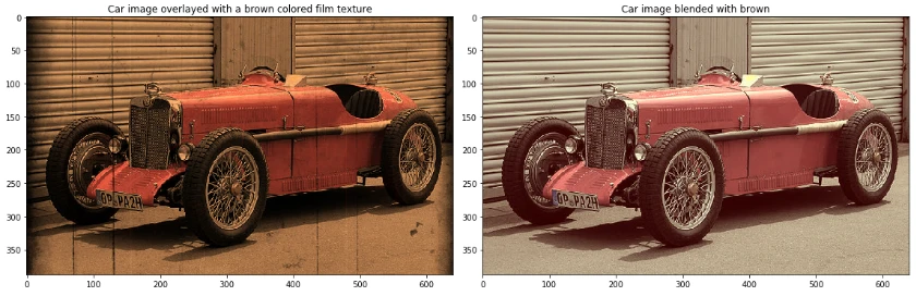
Creating a simple “aged photograph” effect by globally blending the half-desaturated image from the previous step with some amount of brown.

Car image has been blended with brown color and a brown colorized old photo texture.

In [6]:

# source: https://www.photoshopsupply.com/patterns-textures/free-dust-textures# license: https://www.photoshopsupply.com/license# This file is free for Personal and Commercial use with attribution.!wget https://www.photoshopsupply.com/wp-content/uploads/2019/07/film-texture-1.jpg -O film-texture-1.jpg

--2022-07-20 20:50:59--  https://www.photoshopsupply.com/wp-content/uploads/2019/07/film-texture-1.jpg
Resolving www.photoshopsupply.com (www.photoshopsupply.com)... 104.21.61.201, 172.67.214.71, 2606:4700:3032::6815:3dc9, ...
Connecting to www.photoshopsupply.com (www.photoshopsupply.com)|104.21.61.201|:443... connected.
HTTP request sent, awaiting response... 200 OK
Length: 48991 (48K) [image/jpeg]
Saving to: ‘film-texture-1.jpg’

film-texture-1.jpg  100%[===================>]  47,84K  --.-KB/s    in 0,001s  

2022-07-20 20:51:00 (81,7 MB/s) - ‘film-texture-1.jpg’ saved [48991/48991]

In [7]:

f, (ax1, ax2) = plt.subplots(1, 2, figsize=(16,12))# Load film texturefilm_texture = Image.open("film-texture-1.jpg")film_texture = film_texture.resize((rgb_data.shape[1], rgb_data.shape[0])) # resize the image as same as the car imagefilm_texture = np.array(film_texture)/255.0 # normalize between 0 and 1# brown hsv code: https://en.wikipedia.org/wiki/Brownfilm_texture_hsv = colors.rgb_to_hsv(film_texture)film_texture_hsv[:,:,0] = 30/360film_texture_hsv[:,:,1] = 0.6  # saturation is modified!film_texture_hsv[:,:,2] *= 0.59film_texture_colorized = colors.hsv_to_rgb(film_texture_hsv)_=plt.imshow(film_texture_colorized)ax1.imshow(film_texture)ax1.set_title("Loaded film texture")ax2.imshow(film_texture_colorized)ax2.set_title("Colorized film texture")f.tight_layout()

In [8]:

# https://en.wikipedia.org/wiki/Blend_modes#Overlay# a is base layer, b is top layerdef overlay(a,b):    mask = a < 0.5    c = a.copy()    c[mask] = 2 * a[mask] * b[mask]    c[~mask] = 1 - 2*(1-a[~mask]) * (1-b[~mask])    return c# Create only brown imagebrown_hsv = film_texture_hsv.copy()brown_hsv[:,:,0] = 30/360brown_hsv[:,:,1] = 0.3  # saturation is modified!brown_hsv[:,:,2] = 0.59brown_rgb = colors.hsv_to_rgb(brown_hsv)f, (ax1, ax2) = plt.subplots(1, 2, figsize=(16,12))new_image1 = overlay(film_texture_colorized, reduced_saturation_img)ax1.imshow(new_image1)ax1.set_title("Car image overlayed with a brown colored film texture")new_image2 = overlay(brown_rgb, reduced_saturation_img)ax2.imshow(new_image2)ax2.set_title("Car image blended with brown")f.tight_layout()

Rotating the hues of the original image so that the car obtains a different color. Provide two images in which the car is blue, and has another color of your choice.

In [9]:

rotate_for_blue = 0.6img = colors.rgb_to_hsv(rgb_data)modified_hsv = img.copy()modified_hsv[:,:,0] += rotate_for_bluemodified_hsv[:,:,0] %= 1.0new_rgb_image = colors.hsv_to_rgb(modified_hsv)plt.imshow(new_rgb_image)_ = plt.title("rotated hue: " + str(rotate_for_blue) + " - Blue")

In [10]:

from matplotlib.animation import FuncAnimationfrom IPython.display import HTMLfig, ax = plt.subplots(figsize=(9,6))def update(frame):    img = colors.rgb_to_hsv(rgb_data)    modified_hsv = img.copy()    modified_hsv[:,:,0] += frame    modified_hsv[:,:,0] = modified_hsv[:,:,0] % 1.0    new_rgb_image = colors.hsv_to_rgb(modified_hsv)    plt.imshow(new_rgb_image)    plt.title("rotated hue: " + str(round(frame,2)))ani = FuncAnimation(fig, update, frames=np.linspace(0, 1, 40), blit=False)video = ani.to_html5_video()plt.close()HTML(video)

Out[10]:

Manipulating the hue values of only those pixels which show a pinkish / purplelish hue such that their hue becomes yellowish. (In plainer Englisher: implement code that makes the flow yellow.)

In [11]:

img = cv2.imread("Data/colored_flower.png")hsv_img = cv2.cvtColor(img, cv2.COLOR_BGR2HSV)fig, (ax1, ax2) = plt.subplots(1, 2, figsize=(12,12))_ = ax1.imshow(img); _ = ax1.set_title("RGB image")_ = ax2.imshow(hsv_img); _ = ax2.set_title("HSV image")

In [12]:

#hsv_img = np.array(hsv_img)h = hsv_img[:,:,0]s = hsv_img[:,:,1]v = hsv_img[:,:,2]#_ = plt.imshow(img); _ = plt.title("original image")fig, (ax1, ax2, ax3) = plt.subplots(1, 3, figsize=(25,25))_ = ax1.imshow(h); _ = ax1.set_title("hue channel")_ = ax2.imshow(s, cmap="gray"); _ = ax2.set_title("saturation channel")_ = ax3.imshow(v, cmap="gray"); _ = ax3.set_title("value channel")

The hue range of reddish/pinkish/purplish color is [240,360]. In this flower image, the flower is more pinkish, and considering the hue ranges of colors, shifting 120 degrees the hue values of pinkish parts of the image will make the flower look yellowish. Since the hue range of OpenCV ranges between [0,180], the hue range of reddish/pinkish/purplish color is approximately [120,180] and 60 degrees shifting can be applied to obtain yellowish color.
The following two cells show the ways of shifting the color of the flower. The former cell uses a mask while the latter employs np.where method.

In [13]:

mask = h>120modified_hsv_img = hsv_img.copy()modified_hsv_img[:,:,0][mask] = hsv_img[:,:,0][mask] + 60modified_img = cv2.cvtColor(modified_hsv_img, cv2.COLOR_HSV2RGB)fig, (ax1, ax2, ax3) = plt.subplots(1,3,figsize=(15,15))_ = ax1.imshow(img); _ = ax1.set_title("original image")_ = ax2.imshow(mask, cmap="gray"); _ = ax2.set_title("mask")_ = ax3.imshow(modified_img); _ = ax3.set_title("yellowish image")

In [14]:

yellowish_hue = np.where(h>120, (h+60)%180, h)modified_hsv_img = hsv_img.copy()modified_hsv_img[:,:,0] = yellowish_huemodified_img = cv2.cvtColor(modified_hsv_img, cv2.COLOR_HSV2RGB)fig, (ax1, ax2) = plt.subplots(1,2,figsize=(10,10))_ = ax1.imshow(img); _ = ax1.set_title("original image")_ = ax2.imshow(modified_img); _ = ax2.set_title("yellowish image")

In [15]:

img = cv2.imread("Data/reddish_img.jpg")   #opencv uses BGR color as a default color space to display imageshsv_img = cv2.cvtColor(img, cv2.COLOR_BGR2HSV)img = cv2.cvtColor(img, cv2.COLOR_BGR2RGB)h = hsv_img[:,:,0]s = hsv_img[:,:,1]v = hsv_img[:,:,2]fig, (ax1, ax2, ax3) = plt.subplots(1, 3, figsize=(25,25))_ = ax1.imshow(h); _ = ax1.set_title("hue channel")_ = ax2.imshow(s, cmap="gray"); _ = ax2.set_title("saturation channel")_ = ax3.imshow(v, cmap="gray"); _ = ax3.set_title("value channel")mask = ((h>165) | (h<5)) & (s>80) & (v>80)  # Red color parametersmask = mask.astype(np.uint8)*255fig, (ax1, ax2) = plt.subplots(1, 2, figsize=(12,12))_ = ax1.imshow(img); _ = ax1.set_title("original image")_ = ax2.imshow(mask, cmap="gray"); _ = ax2.set_title("mask")