← All notebooks

December 5, 2021 5 min read

Support Vector Machines

Usage of SVM with different kernels on various datasets. SVM with linear kernels, polynomial kernels, RBF kernels, sigmoid kernels are run on datasets and results are shown.

Support Vector Machines¶

Table of Contents

• 1  Support Vector Machines
  • 1.1  Load Dataset
  • 1.2  Scale Dataset
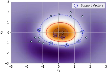
  • 1.3  Example SVM Code with RBF Kernel
  • 1.4  Functionize SVM Scenarios
  • 1.5  Analyzing Assignment 51 Dataset
  • 1.6  Analyzing PA-E_t2
  • 1.7  Analyzing PA-E_t3
  • 1.8  Analyzing PA-E_t4
  • 1.9  Analyzing PA-E_t5
  • 1.10  Analyzing PA-E_t6
  • 1.11  Analyzing PA-E_t7
  • 1.12  Set the parameters by cross-validation

Load Dataset¶

In [1]:

import numpy as npimport matplotlib.pyplot as pltfrom sklearn import svmfrom sklearn.preprocessing import StandardScalerfrom sklearn.model_selection import StratifiedShuffleSplitfrom sklearn.model_selection import GridSearchCVfrom sklearn.svm import SVCimport warningswarnings.filterwarnings('ignore')def load_dataset(filename):    f = open(filename, "r")    dataset = []    skip_first = True    for l in f:        if skip_first:            skip_first = False            continue        txt = l.strip()        a,b,c = txt.split(" ")        b = b.split(":")[1]        c = c.split(":")[1]        dataset.append( [a,b,c] )    dataset = np.array(dataset, dtype=np.float)    dataset_x = dataset[:, 1:]    dataset_y = dataset[:, 0]    return dataset_x, dataset_y# Datasetsdataset2_x, dataset2_y = load_dataset("data/PA-E_t2.txt")dataset3_x, dataset3_y = load_dataset("data/PA-E_t3.txt")dataset4_x, dataset4_y = load_dataset("data/PA-E_t4.txt")dataset5_x, dataset5_y = load_dataset("data/PA-E_t5.txt")dataset6_x, dataset6_y = load_dataset("data/PA-E_t6.txt")dataset7_x, dataset7_y = load_dataset("data/PA-E_t7.txt")# Datasetdataset51_x = np.array([[0, 3], [1, 3], [1, 2], [2, 2], [2, 4], [5, 8], [0, -3], [1, -3], [1, -2], [2, -4], [3, 1], [3, 0], [3, -2], [4, -1], [5, 1]])dataset51_y = np.array([-1,-1,-1,-1,-1,-1,1,1,1,1,1,1,1,1,1])

Scale Dataset¶

In [2]:

# Scale dataset to mean=0 variance=1scaler2 = StandardScaler()dataset2_x_scaled = scaler2.fit_transform(dataset2_x)scaler3 = StandardScaler()dataset3_x_scaled = scaler3.fit_transform(dataset3_x)scaler4 = StandardScaler()dataset4_x_scaled = scaler4.fit_transform(dataset4_x)scaler5 = StandardScaler()dataset5_x_scaled = scaler5.fit_transform(dataset5_x)scaler6 = StandardScaler()dataset6_x_scaled = scaler6.fit_transform(dataset6_x)scaler7 = StandardScaler()dataset7_x_scaled = scaler7.fit_transform(dataset7_x)scaler51 = StandardScaler()dataset51_x_scaled = scaler51.fit_transform(dataset51_x)_=plt.scatter(dataset7_x_scaled[:,0], dataset7_x_scaled[:,1], s=100, c=dataset7_y)_=plt.xlabel("$x_1$")_=plt.ylabel("$x_2$")_=plt.title("Dataset scaled with StandartScaler")

Example SVM Code with RBF Kernel¶

In [3]:

# Fit the modelclf = svm.SVC(kernel='rbf', C=10000)clf.fit(dataset7_x_scaled, dataset7_y)# Prepare the figureplt.grid(True)plt.xlabel("$x_1$")plt.ylabel("$x_2$")# Plot the decision function for each datapoint on the gridxx, yy = np.meshgrid(np.linspace(-3, 3, 500),                    np.linspace(-3, 3, 500))Z = clf.decision_function(np.c_[xx.ravel(), yy.ravel()])Z = Z.reshape(xx.shape)# Plot model output for every pixel on the figureplt.imshow(Z, interpolation='nearest', extent=(xx.min(), xx.max(), yy.min(), yy.max()), aspect='auto', origin='lower', cmap=plt.cm.PuOr_r)# Plot decision boundaryplt.contour(xx, yy, Z, colors='r', levels=[0], alpha=0.75,           linestyles=['-'])plt.contour(xx, yy, Z, colors='b', levels=[-1, 1], alpha=0.5,           linestyles=['--', '--'])# Plot support vectorsplt.scatter(clf.support_vectors_[:, 0], clf.support_vectors_[:, 1], s=150,           linewidth=1, facecolors='none', edgecolors='b', label="Support Vectors")# Plot dataset_=plt.scatter(dataset7_x_scaled[:, 0], dataset7_x_scaled[:, 1], s=30, c=dataset7_y, cmap=plt.cm.Paired, edgecolors='k')_=plt.legend()

Functionize SVM Scenarios¶

In [4]:

def svm_scenario(ax, x, y, zoom, kernel, C, title=None):    # Fit the model    clf = svm.SVC(kernel=kernel, C=C)    clf.fit(x, y)    # Plot results    if ax is not None:        # Prepare the figure        ax.grid(True)        ax.set_xlabel("$x_1$")        ax.set_ylabel("$x_2$")        if title is not None:            ax.set_title(title)        # Plot the decision function for each datapoint on the grid        xlim = [np.min(x[:,0])-zoom ,np.max(x[:,0])+zoom]        ylim = [np.min(x[:,1])-zoom ,np.max(x[:,1])+zoom]        xx, yy = np.meshgrid(np.linspace(xlim[0], xlim[1], 100),                            np.linspace(ylim[0], ylim[1], 100))        zz = clf.decision_function(np.c_[xx.ravel(), yy.ravel()])        zz = zz.reshape(xx.shape)        # Plot model output for every pixel on the figure        ax.imshow(zz, interpolation='nearest', extent=(xx.min(), xx.max(), yy.min(), yy.max()), aspect='auto', origin='lower', cmap=plt.cm.PuOr_r)        # Plot decision boundary        ax.contour(xx, yy, zz, colors='r', levels=[0], alpha=0.75, linestyles=['-'])        ax.contour(xx, yy, zz, colors='b', levels=[-1, 1], alpha=0.5, linestyles=['--', '--'])        # Plot support vectors        ax.scatter(clf.support_vectors_[:, 0], clf.support_vectors_[:, 1], s=150, linewidth=1, facecolors='none', edgecolors='b', label="Support Vectors")        # Plot dataset        ax.scatter(x[:, 0], x[:, 1], s=30, c=y, cmap=plt.cm.Paired, edgecolors='k')        ax.legend()fig, (ax1, ax2) = plt.subplots(1, 2, figsize=(12,6))fig.tight_layout()svm_scenario(ax=ax1, x=dataset7_x_scaled, y=dataset7_y, zoom=1, kernel='rbf', C=1000, title="RBF Kernel, C=1000")svm_scenario(ax=ax2, x=dataset7_x_scaled, y=dataset7_y, zoom=1, kernel='rbf', C=1, title="RBF Kernel, C=1")

Analyzing Assignment 51 Dataset¶

In [5]:

kernels=["linear", "poly", "rbf", "sigmoid"]c_values = [0.1, 1, 10, 100] # Regularization parameter. The strength of the regularization is inversely proportional to C. Must be strictly positive. The penalty is a squared l2 penalty.fig, axs = plt.subplots(len(c_values), len(kernels), figsize=(24,15))for i,k in enumerate(kernels):    for j,c in enumerate(c_values):        svm_scenario(ax=axs[j,i], x=dataset51_x_scaled, y=dataset51_y, zoom=1, kernel=k, C=c, title=k+" kernel, C="+str(c))fig.tight_layout()

Analyzing PA-E_t2¶

In [6]:

kernels=["linear", "poly", "rbf", "sigmoid"]c_values = [0.1, 1, 10, 100] # Regularization parameter. The strength of the regularization is inversely proportional to C. Must be strictly positive. The penalty is a squared l2 penalty.fig, axs = plt.subplots(len(c_values), len(kernels), figsize=(24,15))for i,k in enumerate(kernels):    for j,c in enumerate(c_values):        svm_scenario(ax=axs[j,i], x=dataset2_x_scaled, y=dataset2_y, zoom=1, kernel=k, C=c, title=k+" kernel, C="+str(c))fig.tight_layout()

Analyzing PA-E_t3¶

In [7]:

kernels=["linear", "poly", "rbf", "sigmoid"]c_values = [0.1, 1, 10, 100] # Regularization parameter. The strength of the regularization is inversely proportional to C. Must be strictly positive. The penalty is a squared l2 penalty.fig, axs = plt.subplots(len(c_values), len(kernels), figsize=(24,15))for i,k in enumerate(kernels):    for j,c in enumerate(c_values):        svm_scenario(ax=axs[j,i], x=dataset3_x_scaled, y=dataset3_y, zoom=1, kernel=k, C=c, title=k+" kernel, C="+str(c))fig.tight_layout()

Analyzing PA-E_t4¶

In [8]:

kernels=["linear", "poly", "rbf", "sigmoid"]c_values = [0.1, 1, 10, 100] # Regularization parameter. The strength of the regularization is inversely proportional to C. Must be strictly positive. The penalty is a squared l2 penalty.fig, axs = plt.subplots(len(c_values), len(kernels), figsize=(24,15))for i,k in enumerate(kernels):    for j,c in enumerate(c_values):        svm_scenario(ax=axs[j,i], x=dataset4_x_scaled, y=dataset4_y, zoom=1, kernel=k, C=c, title=k+" kernel, C="+str(c))fig.tight_layout()

Analyzing PA-E_t5¶

In [9]:

kernels=["linear", "poly", "rbf", "sigmoid"]c_values = [0.1, 1, 10, 100] # Regularization parameter. The strength of the regularization is inversely proportional to C. Must be strictly positive. The penalty is a squared l2 penalty.fig, axs = plt.subplots(len(c_values), len(kernels), figsize=(24,15))for i,k in enumerate(kernels):    for j,c in enumerate(c_values):        svm_scenario(ax=axs[j,i], x=dataset5_x_scaled, y=dataset5_y, zoom=1, kernel=k, C=c, title=k+" kernel, C="+str(c))fig.tight_layout()

Analyzing PA-E_t6¶

In [10]:

kernels=["linear", "poly", "rbf", "sigmoid"]c_values = [0.1, 1, 10, 100] # Regularization parameter. The strength of the regularization is inversely proportional to C. Must be strictly positive. The penalty is a squared l2 penalty.fig, axs = plt.subplots(len(c_values), len(kernels), figsize=(24,15))for i,k in enumerate(kernels):    for j,c in enumerate(c_values):        svm_scenario(ax=axs[j,i], x=dataset6_x_scaled, y=dataset6_y, zoom=1, kernel=k, C=c, title=k+" kernel, C="+str(c))fig.tight_layout()

Analyzing PA-E_t7¶

In [11]:

kernels=["linear", "poly", "rbf", "sigmoid"]c_values = [0.1, 1, 10, 100] # Regularization parameter. The strength of the regularization is inversely proportional to C. Must be strictly positive. The penalty is a squared l2 penalty.fig, axs = plt.subplots(len(c_values), len(kernels), figsize=(24,15))for i,k in enumerate(kernels):    for j,c in enumerate(c_values):        svm_scenario(ax=axs[j,i], x=dataset7_x_scaled, y=dataset7_y, zoom=1, kernel=k, C=c, title=k+" kernel, C="+str(c))fig.tight_layout()

Mostly linear and rbf kernels worked well with all the data. Even tough C value is default 1, higher values seem to work better.

In [13]:

datasetTest_x, datasetTest_y = load_dataset("data/PA-E_Test.txt")_=plt.scatter(datasetTest_x[:,0], datasetTest_x[:,1], s=100, c=datasetTest_y)_=plt.xlabel("$x_1$")_=plt.ylabel("$x_2$")

Set the parameters by cross-validation¶

In [15]:

X, Y = load_dataset("data/PA-E_t7.txt")C_values = 10**np.linspace(-3, 3, 14)G_values = 10**np.linspace(-3, 3, 7)tuned_parameters = [{'kernel': ['rbf'],     'C': C_values, 'gamma': G_values},                    {'kernel': ['linear'],  'C': C_values},                    {'kernel': ['poly'],    'C': C_values},                    {'kernel': ['sigmoid'], 'C': C_values}]scores = ['precision', 'recall']for score in scores:    print("# Tuning hyper-parameters for %s" % score)    clf = GridSearchCV(        SVC(), tuned_parameters, scoring='%s_macro' % score    )    clf.fit(X, Y)    print("Best parameters set found on development set:")    print(clf.best_params_)    #print("Grid scores on development set:")    #print()    #means = clf.cv_results_['mean_test_score']    #stds = clf.cv_results_['std_test_score']    #for mean, std, params in zip(means, stds, clf.cv_results_['params']):    #    print("%0.3f (+/-%0.03f) for %r"    #          % (mean, std * 2, params))    #print()

# Tuning hyper-parameters for precision
Best parameters set found on development set:
{'C': 0.5878016072274912, 'gamma': 0.1, 'kernel': 'rbf'}
# Tuning hyper-parameters for recall
Best parameters set found on development set:
{'C': 0.5878016072274912, 'gamma': 0.1, 'kernel': 'rbf'}

Used: https://scikit-learn.org/stable/modules/svm.html